Measuring Impedances with an Oscilloscope

Measuring impedances of electrical components can be done with high precision results using an oscilloscope and a measuring transmitter. For this purpose we present a method that converts measurement data in a spreadsheet such as Excel. More advanced evaluations are possible with curve sample data and statistical software packages such as R, Python or Matlab.

Firstly, the method described determines the inductances or capacitances of unknown components. It is also suitable for measuring frequency responses when the actual impedances deviate significantly from theoretical values in high-frequency applications. The latter is a common problem in high-frequency technology, if only because real components are always lossy.

If you are familiar with the theory of reactance and complex numbers, you can skip the following sections and continue with the test setup for measuring impedances.

Impedances of Ideal Inductors and Capacitors

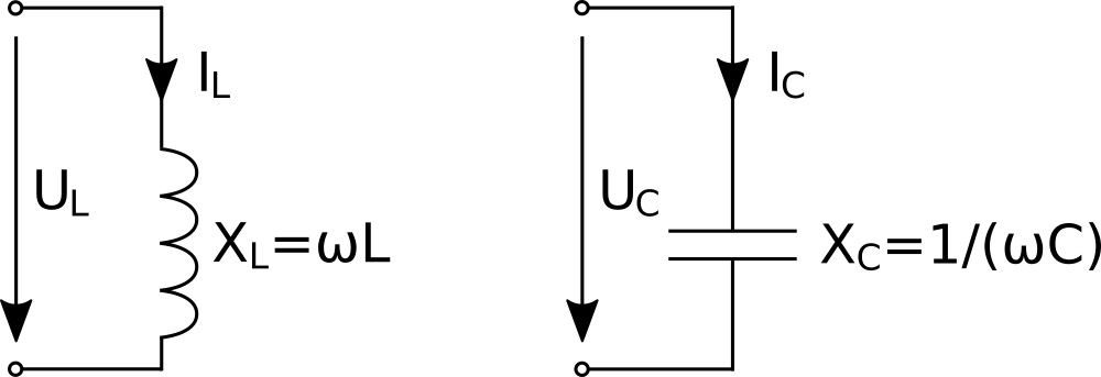
The impedances XL and XC of ideal inductors and capacitors follow from two simple formulas. For both of them, current and voltage are 90° out of phase.

XL = ω*L
XC = 1/(ω*C)
ω = 2*π*f

L: inductance in Henry
C: capacity in Farad
f: frequency in Hertz
XL: impedance of an ideal inductor
XC: impedance of an ideal capacitor

With ideal inductors, the voltage UL leads the current IL by 90°. It’s the reverse for ideal capacitors, where the voltage UC lags the current IC by 90°.

As a consequence of 90° phase shifts, ideal capacitors and inductors function as reactances. This means that unlike ohmic resistances, they don’t consume any power. Instead, they periodically store and release energy.

If the phase shifts are close to these ideal values, determining the inductance and capacitance of elements is simple. In that case, it is sufficient to just measure the amounts of currents and voltages along the components. Afterwards, the sought-for characteristics follow from these simple computations:

XL = |UL| / |IL|
XC = |UC| / |IC|
L = XL / ω
C = 1 / (ω*XC)

Impedances of Real Inductors and Capacitors

Equivalent circuit diagrams of real coils and capacitors have ohmic resistances added in parallel and series circuits.

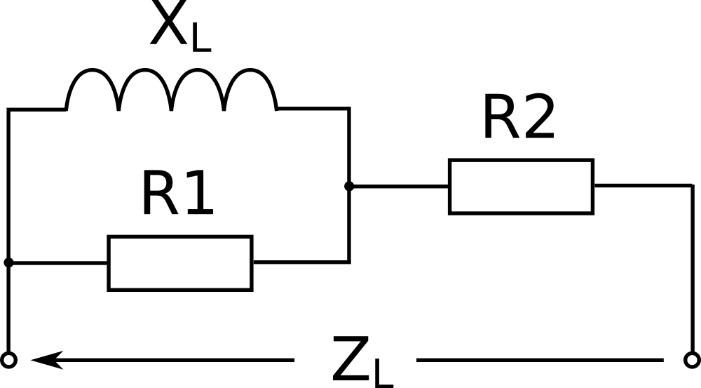
The equivalent circuit above shows such damping resistances for a lossy coil. To obtain an equivalent circuit diagram for capacitors instead, simply swap XL and ZL for XC and ZC. In most cases, equivalent circuits with only one damping resistor are sufficient. We can then assume that either R1→∞ or R2=0.

Because of more complex networks, phasor diagrams are helpful measuring impedances ZC and ZL of lossy real components. Such phasor diagrams are complex number representations of amount and phase of alternating currents and alternating voltages. If you are not familiar with them, you could read the article on alternating currents in the complex number plane.

Test Setup for Measuring Impedances

The test setup for measuring impedances comprises the following equipment: a two-channel oscilloscope, a measurement generator or measurement transmitter, and software to convert and evaluate results. For the conversions spreadsheets such as Excel or LibreOffice are great. Statistical software packages such as R, Python or Matlab also perform more advanced evaluations.

With digital oscilloscopes that store measurement data in file formats for import into Excel, R or Matlab, the evaluation is much simpler and more precise. However, the circuits for measuring the components remain the same.

There are two measurement variants. The first of which determines the current flow through the impedance and the second the voltage drop across it. Variant 1 suits large impedances and variant 2 is better for small ones.

Variant 1: Measuring Impedances with an Oscilloscope Observing the Current Flow

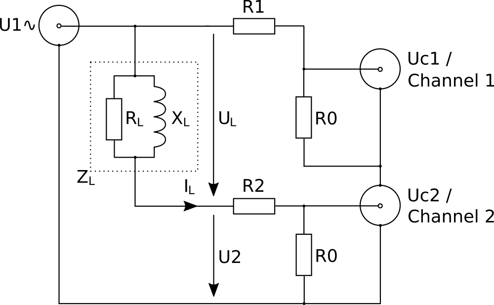
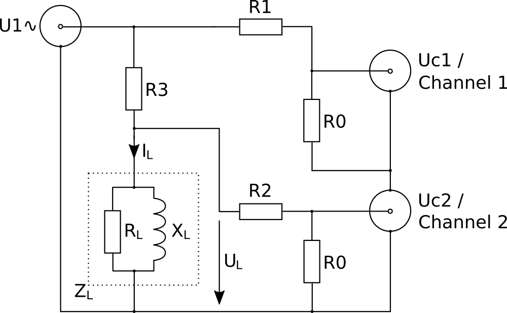
Figure 3 shows the circuit for measuring impedances via the current IL flowing through the component. Two channels of the oscilloscope, equipped with voltage dividers, record the high-frequency input signal U1 and the secondary voltage U2. The current IL then follows from U2.

First of all, voltage dividers precede the channels of the oscilloscope. Otherwise the capacitances of the measurement inputs would falsify the results. In a test setup with 50Ω coaxial cable, a low value of around 50Ω is suitable for the parallel resistance R0. This corresponds to the line impedances and also reduces the influence of the capacitance of the measurement input connected in parallel.

In order to further reduce distortions caused by input capacitances, the resistors R1 and R2 should also be significantly larger than R0. Values of at least 500Ω are then recommended.

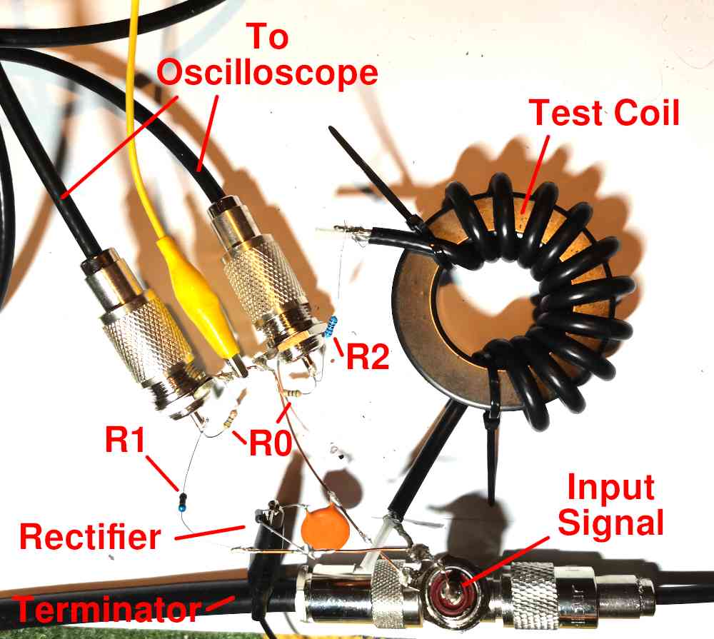
Figure 4 shows an experimental setup corresponding to the components of the circuit in Figure 3. The additional rectifier installed to measure the amplitude of the input signal is optional. Furthermore, the setup includes a 50Ω terminating resistor protecting the transmitter. As the specific experiment was about measuring the impedance of a shield wave barrier, the test coil is wound with coaxial cable. To not falsify the phases when measuring high-frequency signals, the two cables to the oscilloscope should have equal lengths.

Measurement Method for Variant 1

The oscilloscope is measuring the voltages Uc1 and Uc2 on channels 1 and 2. From the voltage dividers R1/R0 and R2/R0 we get the input signal U1 and the secondary voltage U2. The current IL through the component then follows from U2 and R2/R0:

U1 = Uc1 * (R1 + R0) / R0
U2 = Uc2 * (R2 + R0) / R0
IL = U2 / (R2 + R0)

For impedance measurement we need UL and IL. While is IL simply a conversion of the voltage on channel 2, UL only follows from the difference between U1 and U2:

UL = U1 - U2

However, due to the phase shifts in the circuit, the differential voltage UL cannot be determined from the difference in the amplitudes or amounts of the voltages U1 and U2!

|UL| ≠ |U1| - |U2|

It’s best to look at this fact and phase shifts that are important for measuring impedances in phasor diagram.

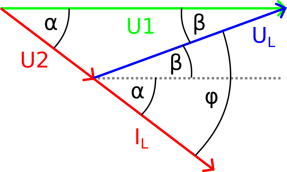
As can be seen in Figure 5, the voltage U2 and current IL lag behind the input voltage U1 by a phase angle α. The voltage UL, on the other hand, leads the input voltage U1 by an angle β. As indicated by the gray dotted line parallel to U1, the angles α and β add up to the phase shift φ between IL and UL.

The following restrictions apply to the phase shift φ of a real coil and the phase angle α: φ<90° and α<φ. Therefore, even with an ideal coil the phase shift α observed on channel 2 of the oscilloscope is less than 90°!

The following calculations each refer to the vector lengths or magnitudes of the voltages and currents in the vector diagram. For the sake of simplicity, I refrain from marking amounts, so I write UL instead of |UL|, for example.

Using the voltage U2 with phase angle α observed on channel 2 of the oscilloscope, we can first calculate the voltage UL. With the cosine law of geometry applies:

UL2 = U12 + U22 - 2 * U1 * U2 * cos(α)
or
UL = sqrt( U12 + U22 - 2 * U1 * U2 * cos(α) )

The angle β now follows from UL with the reversal of the law of cosines:

β = arccos( (UL2 + U12 - U22)/(2 * U1 * UL) )

From the trigonometry of the complex number plane diagram, we now have all the quantities we need to calculate the impedance ZL.

ZL = UL / IL
φ = α + β

ZL: magnitude of impedance of the coil
φ: phase shift UL to IL

For an ideal coil, the angle φ is 90° and for a heavily damped coil it approaches 0°. Finally we can calculate the values of RL and XL of the equivalent circuit.

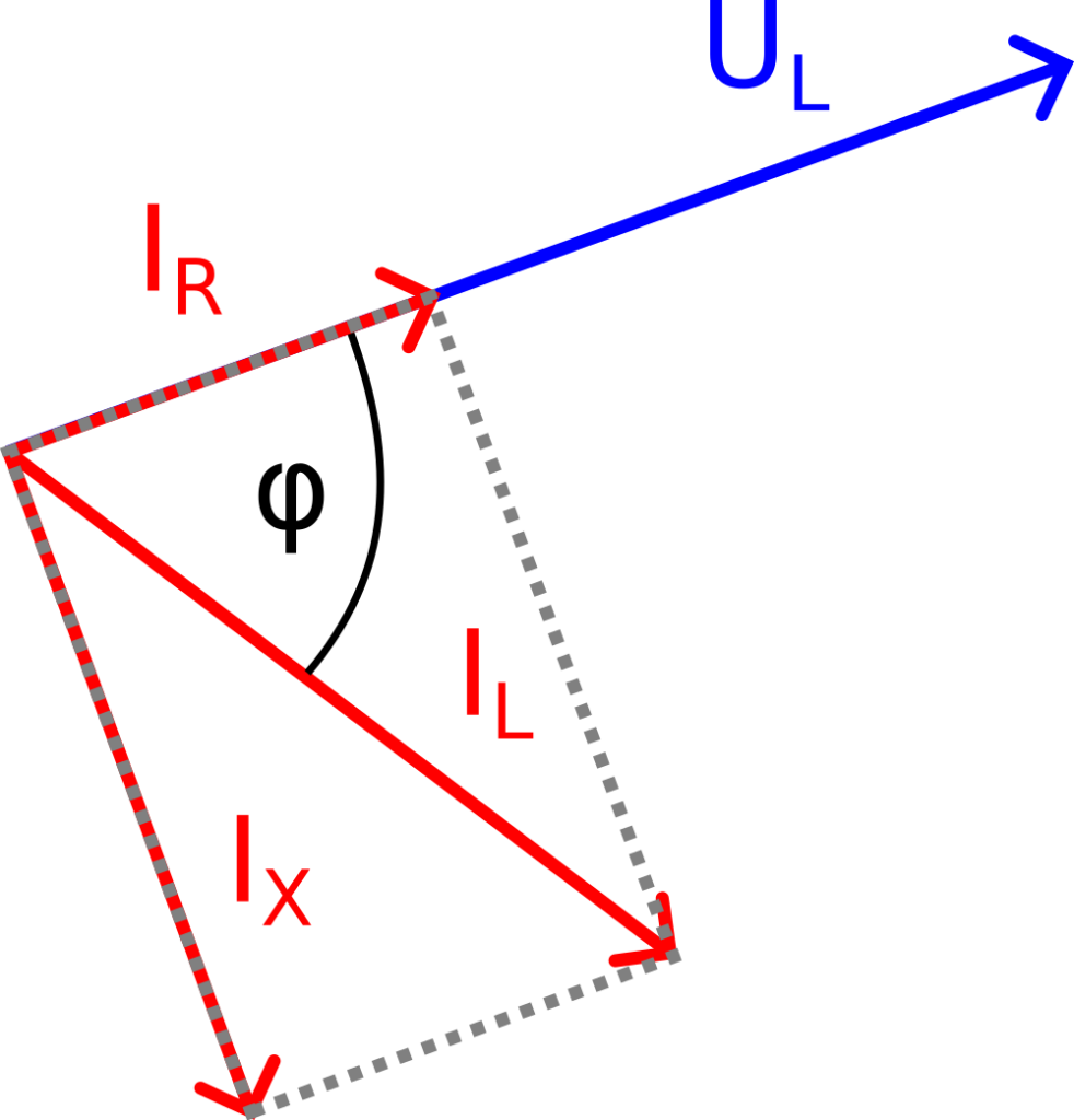
Because of the parallel connection of the real resistance RL and reactance XL, their values are best determined from the active and reactive components of the current I_L. We can visualize them by inserting a rectangle spanned by IL into the phasor diagram. The resulting components IR and IX as shown in Figure 6 then follow from these formulas:

IR = IL * cos(φ)
IX = IL * sin(φ)
RL = UL / IR
XL = UL / IX

Summary Variant 1 for Measuring Impedances Observing the Current

In summary, the component impedance ZL results from the following non-linear system of equations:

U1 = Uc1 * (R1 + R0) / R0
U2 = Uc2 * (R2 + R0) / R0
IL = U2 / (R2 + R0)
UL = sqrt( U12 + U22 - 2 * U1 * U2 * cos(α) )
β = arccos( (UL2 + U12 - U22)/(2 * U1 * UL) )
ZL = UL / IL
φ = α + β
IR = IL * cos(φ)
IX = IL * sin(φ)
RL = UL / IR = ZL / cos(φ)
XL = UL / IX = ZL / sin(φ)

Input variables:
Uc1: Signal at channel 1
Uc2: Signal at channel 2
α: Phase shift Uc1, Uc2
R0, R1, R2: Resistors of voltage dividers

Results for the coil:
ZL: Amount of impedance
φ: Phase shift of impedance
RL: Damping resistance
XL: Reactance

Using Excel it’s easy to solve the system of equations. For each measurement, simply put all intermediate results in separate columns to reference them in the next equation.

Variant 2: Measuring Impedances with an Oscilloscope Observing the Voltage Drop

In variant 2 of the test setup, we observe the voltage drop UL at the coil, but we need to compute the current IL flowing through the coil. First of all, the following applies to the voltages U1 and UL:

U1 = Uc1 * (R1 + R0) / R0
UL = Uc2 * (R2 + R0) / R0

Next, there is an equivalent circuit diagram of the coil ZL and the resistors R1, R2 and R3 that simplifies computations:

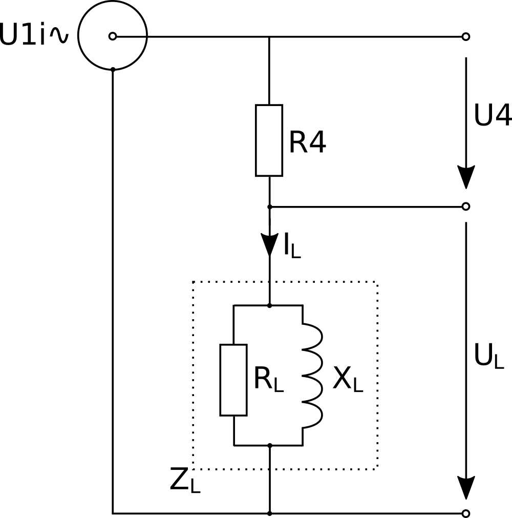
The equivalent circuit converts the voltage divider of R3 and R2+R0 into the internal resistance R4 of an ideal voltage source. It thus eliminates resistors R2+R0 parallel to the sought-for impedance ZL. The following transformations are necessary for this simplification:

U1i = U1 * (R2 + R0) / (R3 + R2 + R0)
R4 = (R2 + R0) * R3  / (R3 + R2 + R0)

So the internal resistance R4 of the ideal source U1i is a parallel connection of resistances R3 and R2+R0. With the equivalent circuit shown in Figure 8, the current IL is:

U4 = U1i - UL
IL = U4 / R4

Because of the phase shifts in the circuit, however, the voltage U4 is not the same as the difference between the magnitudes of the voltages U1i and UL.

|U4| ≠ |U1i| - |UL|

Again, a phasor diagram is employed for clarification. In the following, I omit the identification of amounts, so I write U4 instead of |U4|, for example.

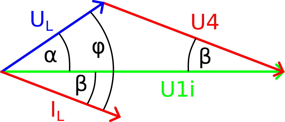
As before, we get the voltage U4 via the phase α and the law of cosines.

U4 = sqrt( UL2 + U1i2 - 2 * UL * U1i * cos(α) )

The phase angle β now follows from U4 and the reversal of the law of cosines.

β = arccos( (U42 + U1i2 - UL2)/(2 * U4 * U1i) )

Because the current IL runs in phase with the voltage drop U4 at R4, the phase angles β replicate themselves in the diagram. This gives us the magnitude and phase of IL:

IL = U4 / R4
φ = α + β

Analogous to the solution for variant 1, we now calculate the active and reactive components of the impedance ZL:

ZL = UL / IL
IR = IL * cos(φ)
IX = IL * sin(φ)
RL = UL / IR = ZL / cos(φ)
XL = UL / IX = ZL / sin(φ)

Summary Variant 2 for Measuring Impedances Observing the Voltage Drop

As before in variant 1, the solution is given in form of a non-linear system of equations:

U1 = Uc1 * (R1 + R0) / R0
UL = Uc2 * (R2 + R0) / R0
U1i = U1 * (R2 + R0) / (R3 + R2 + R0)
R4 = (R2 + R0) * R3  / (R3 + R2 + R0)
U4 = sqrt( UL2 + U1i2 - 2 * UL * U1i * cos(α) )
β = arccos( (U42 + U1i2 - UL2)/(2 * U4 * U1i) )
IL = U4 / R4
φ = α + β
ZL = UL / IL
IR = IL * cos(φ)
IX = IL * sin(φ)
RL = UL / IR = ZL / cos(φ)
XL = UL / IX = ZL / sin(φ)

Input variables:
Uc1: Signal at channel 1
Uc2: Signal at channel 2
α: Phase shift Uc1, Uc2
R0, R1, R2, R3: Resistors of voltage dividers

Results:
ZL: Amount of impedance
φ: Phase shift of impedance
RL: Damping resistance
XL: Reactance

In variant 2, the system of equations is also solved in Excel. Again, simply put intermediate results in separate columns for reference in subsequent equations.

References

Law of Cosines: Wikipedia.org

Phasor Diagrams: Wikipedia.org

Related Content

Measuring Impedances with an Oscilloscope in German: mantelwelle.de